Web traffic forecasting - FB Prophet vs ARIMA

2021-09-14

8 minute read

Introduction

Time series forecasting is a technique that predicts the future basing on the trends of the past. Many times it is very valuable knowledge for the business, for example, it is easier to plan how many products the company will sell or how many users will visit the website. In this post, I’m going to use Facebook Prophet and ARIMA to predict how many pages views the e-commerce store is going to generate in the next 30 days and compare the results. The objective of the post is to show basic time series forecasting for a common business problem.

In short, ARIMA and Prophet are both really popular methods for time series forecasting. In the case of an e-commerce store probably the most correct approach would be forecasting the number of transactions, but predicting web traffic like page views is in my opinion the most common issue in web analytics. For example, the company can acquire information that will help in deciding on upgrading the servers or not (I do not think that Google has such a problem, but it is just an example case and their public dataset is well prepared). ARIMA (Autoregressive Integrated Moving Average) is a form of regression analysis. The key aspects of the method can be revealed by decomposing the acronym:

AR (autoregression) - the model uses a dependent relationship between an observation and some number of lagged observations,
I (integrated) - differencing of the raw observations to make time-series stationary,
MA (moving average) - the model uses the dependency between an observation and a residual error from a moving average model applied to lagged observations.

The components are specified in the model as parameters. The standard notation for ARIMA is p, d, q, which are substituted with integers to indicate the type of ARIMA model used:

p - number of lag observations in the model,
d - number of times that the raw observation are differenced,
q - the size of the moving average window.

The general equation of the ARIMA is:

ŷt = μ + ϕ1 yt-1 +………+ ϕp yt-p — θ1et-1 -………- θqet-q,

where:

μ → constant,
ϕ1 yt-1 +…+ ϕp yt-p → AR terms (lagged values of y),
-θ1et-1 -………- θqet-q → MA terms (lagged errors).

The prophet is a procedure for forecasting time series data based on an additive model where non-linear trends are fit with yearly, weekly, and daily seasonality, plus holiday effects. It works best with time series that have strong seasonal effects and several seasons of historical data. Prophet is robust to missing data and shifts in the trend, and typically handles outliers well. Its core is the sum of three functions:

y(t) = g(t) + s(t) + h(t) + ϵt,

where:

g(t) - growth,
s(t) - seasonality,
h(t) - holidays,
ϵt - error.

Of course, the presented descriptions of both methods are so short (otherwise it could take dozens of pages) and not so perfect. I do not think there is the possibility to understand them completely without further reading.

The dataset used in the blog post is from google cloud marketplace. The dataset provides 12 months of Google Analytics data from the Google Merchandise Store. There are pieces of information about website traffic, behavior of users, transactions, of course, everything obfuscated to hide sensitive data.

Data

Firstly I’m going to download important libraries and acquire the data. Google Analytics sample dataset is stored in bigquery, so it can be done by connecting with bigquery api, querying a dataset with a simple sql, and saving the result to pandas dataframe. The alternative path would be just typing a query in google cloud console and saving the result to csv.

import pandas as pd
import seaborn as sns
from pmdarima import auto_arima                        
from statsmodels.tools.eval_measures import rmse
from google.cloud import bigquery
from matplotlib import pyplot as plt
from prophet import Prophet
from IPython.core.interactiveshell import InteractiveShell


InteractiveShell.ast_node_interactivity = "all"
plt.style.use("dark_background")
plt.rcParams["figure.figsize"] = (10, 5)

client = bigquery.Client.from_service_account_json('google-credentials.json')
query = """
SELECT
  date,
  SUM(totals.pageviews) AS page_views,
  FROM
  `bigquery-public-data.google_analytics_sample.ga_sessions_*`
GROUP BY
  1
ORDER BY
  1 
  """
  
query_job = client.query(query)
df = query_job.result().to_dataframe()

Querying bigquery datasets using the official client library is an easy task, well described in the google cloud documentation. The second step is to check if NaN values exist in the dataset and change date column type from int to datetime. Facebook Prophet is dealing with missing data and outliers effectively, but I think that is not a bad idea to get rid of them. Datetime type is required by both methods.

df.isna().sum()
df.date = df['date'].apply(pd.to_datetime)

Luckily there are no Nan values in the dataset. Lastly, let’s take a look at a simple plot to check how the data is distributed.

sns.lineplot(data=df, x='date', y='page_views')

{ chart

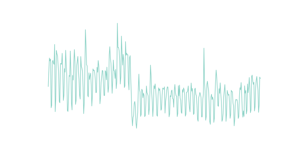
It is noticeable the plot tells us that the time series has a weekly seasonal pattern. I would also assume that there is monthly seasonality.

FB Prophet

The prophet is not so hard tool, I would say it is the easiest one for time series forecasting. Facebook data science teams use it for their own analyses, so after a quick look at the social media rankings, it is easy to say that Prophet is doing the job well.

FB Prophet requires some changes in naming columns in the dataset. Datatime columns have to be ‘ds’, value column needs to be ‘y’. Let’s also create train and test sets.

fbp = df.copy()
fbp.columns = ['ds', 'y']
train_fbp = fbp.iloc[:len(fbp)-30]
test_fbp = fbp.iloc[len(fbp)-30:]

Now it is time to create a model. Prophet follows the sklearn, so everything to do is to create Prophet class and call fit and predict methods. To forecast future web traffic there is the helper method make_future_dataframe. It has specified the number of periods to predict. I’m also going to add the monthly seasonality. In the last step let’s look at the components of the forecast.

m = Prophet()
m.add_seasonality(name='monthly', period=30.5, fourier_order=5)
m.fit(train_fbp)
future = m.make_future_dataframe(periods=30)
forecast = m.predict(future)
m.plot_components(forecast)

{ chart

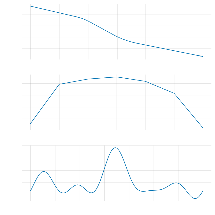
Looking at the components it is possible to confirm that assumption of weekly seasonality was correct. The website has relevantly lower web traffic at the weekends and the peak in the middle of the week. It would be reasonable to advise the marketing team to move more ads budgets to the weekends. The overall trend tends to go down. We can also notice that there might be a montly seasonality, there is a huge peak in the middle of the month.

Next, I’m going to just create a combined dataframe with a test and predicted data and comparison line chart.

fbp_pred = pd.DataFrame({'Date': forecast[-30:]['ds'], 
  "Prediction": forecast[-30:]['yhat']})
fbp_pred = fbp_pred.set_index('Date')
test_fbp['Prediction'] = fbp_pred['Prediction'].values
ax = sns.lineplot(x = test_fbp['ds'], y = test_fbp['y'])
sns.lineplot(x=test_fbp['ds'], y=test_fbp['Prediction'])
plt.legend(labels=['actual', 'predicted'])

{ chart

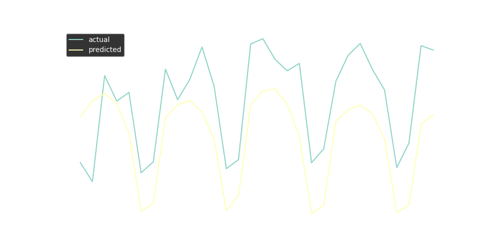
The chart shows that in our case FB Prophet generally predicts the overall trend, but does not handle spikes so well. For being able to compare the model with ARIMA let’s calculate Root Mean Squared Error. RMSE is the square root of the mean of the square of all of the errors. This error metric is a good measure of accuracy for comparing prediction errors of different models or configurations.

fbp_rmse = rmse(test_fbp['y'], test_fbp['Prediction'])
fbp_mean = test_fbp['y'].mean()

print(round(fbp_rmse, 2), round(fbp_rmse/fbp_mean*100, 2))

1977.25 22.03

The RMSE of the model is 1977.25 and it is 22.03% in relation to the mean of the actual values.

ARIMA

To properly implement ARIMA model plenty of steps must be taken. Before fitting the model there is a need to make a series stationary and find p, d, and q values. Fortunately here comes auto_arima. It is a very powerful automation tool, for example, it estimates missing values, detects best p, q, and d values, performs seasonal differencing, makes forecasts. It is of course very short description, more can be read in the documentation.

Firstly, let’s prepare train and test sets, exactly in the same way as for FB Prophet. Next, I’m going to use the auto_arima function. There is a possibility to pass a lot of parameters, I’m not going to do this, because I did not make a lot of changes to basic Prophet also. The most important thing for the discussed dataset is to set the seasonal parameter to True, because of the assumption of the seasonal pattern in the dataset, and m to 7 (for daily data).

ar = df.copy()
ar = ar.set_index('date')
train_ar = ar.iloc[:len(ar)-30]
test_ar = ar.iloc[len(ar)-30:]

model = auto_arima(ar['page_views'], seasonal=True, start_p=0, start_q=0, m=7)
model.summary()

Summary of auto_arima tells us that the best model is SARIMAX(0, 1, 1)x(1, 0, 1, 7). SARIMA models are arima models with seasonal component. They have four additional parameters: seasonal p, d and q (P, D and Q) and m that indicates seasonal length in the data.

Now let’s make and plot the forecast.

forecast = model.predict(n_periods=30)

forecast = pd.DataFrame(forecast, index = test_ar.index,columns=['Prediction'])
plt.plot(test_ar, label='Actual')
plt.plot(forecast, label='Prediction')
plt.legend()
plt.show()

{ chart

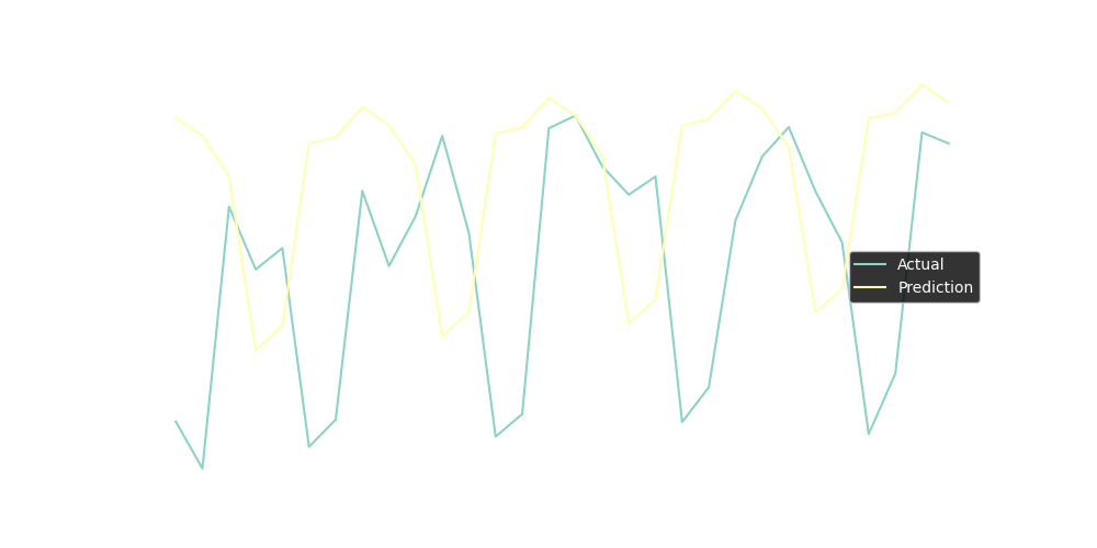
The line chart does not look that bad, but calculating rmse will be better for evaluating and comparing with FB Prophet forecast.

ar_rmse = rmse(test_ar, forecast)[0]
ar_mean = test_ar.mean()[0]
print(round(ar_rmse, 2), round(ar_rmse/ar_mean*100, 2))

2975.42 33.15

The RMSE of the model is 2975.42 and it is 33.15% in relation to the mean of the actual values.

Conclusion

Summing up the experiment it can be noticed that FB Prophet prediction has better accuracy than SARIMA. The normalized RMSE (rmse/mean) for the Prophet is around 22%, meanwhile, SARIMA has nRMSE around 33%

test_fbp = test_fbp.set_index('ds')
plt.plot(test_ar, label='Actual')
plt.plot(forecast, label='SARIMA')
plt.plot(test_fbp['Prediction'], label='FB Prophet')
plt.legend()
plt.show()

{ chart

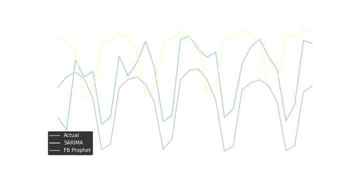
The errors may seem to be huge and Prophet may look much better than SARIMA. However, a few important issues need to be borne in mind. The above experiments just show not so time-consuming and totally basic predictions. Having a better dataset (for example with a longer period), knowledge of the business, or just better tuning the parameters of models could lead to better accuracy or even different conclusion. The goal of the post was to show the basic time series forecasting methods. I believe that the presented methods are useful for businesses, especially online startups. The analysis can be done quickly, using data from Google Analytics, without a lot of data wrangling.

Introduction

Data

FB Prophet

ARIMA

Conclusion

References